Learn SQL Through Football Data
SkillVeris Team
Content Team
SQL is just asking questions of a database in a structured language, and football data makes every query meaningful.
In this guide, you'll learn:
- Five clauses answer almost any football question: SELECT, WHERE, GROUP BY, JOIN, and HAVING.
- A football season is a perfect relational dataset of matches, players, and goals connected by foreign keys.
- WHERE filters rows before grouping while HAVING filters groups after aggregation.
- JOIN links tables by a shared key and is the most powerful operation in SQL.
1Why Football Is Perfect for Learning SQL
A football season generates a perfect relational dataset: matches with one row per game, players with one row per player, and goals with one row per goal event. These tables connect naturally with foreign keys, which makes every SQL concept immediately meaningful.
Instead of 'list all customers who placed more than 3 orders,' you write 'list all players who scored more than 10 goals' and you actually care about the answer.
2Setting Up: SQLite and the Dataset
Download a Premier League dataset from Kaggle by searching 'Premier League SQL' or 'EPL results'. The examples here use three tables that mirror the structure of a real season.
Load the CSV files into SQLite with Python, or use DB Browser for SQLite (free and visual) to import the CSVs and write queries interactively.
- matches: match_id, date, season, home_team, away_team, home_goals, away_goals, result
- players: player_id, name, team, position, nationality
- goals: goal_id, match_id, player_id, minute, goal_type (open play / penalty / own goal)
Load the CSVs into SQLite
A few lines of pandas load each CSV into a SQLite table.
import sqlite3, pandas as pd
conn = sqlite3.connect("football.db")
pd.read_csv("matches.csv").to_sql("matches", conn, if_exists="replace", index=False)
pd.read_csv("players.csv").to_sql("players", conn, if_exists="replace", index=False)
pd.read_csv("goals.csv").to_sql("goals", conn, if_exists="replace", index=False)
print("Database ready")3SELECT and WHERE: Your First Queries
SELECT chooses the columns you want and WHERE filters the rows. Together they answer most basic football questions, from listing a season's fixtures to finding a single team's home matches.
You can also compute new columns inline, such as total goals per match, and filter on them.
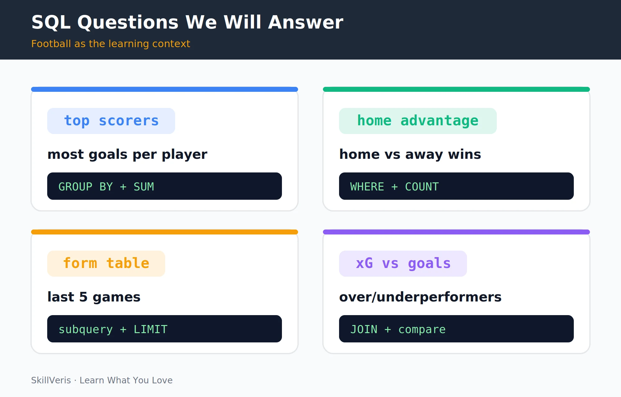
Filtering matches
Pick columns, filter by season and team, and rank high-scoring games.
-- All matches in the 2023/24 season
SELECT date, home_team, away_team, home_goals, away_goals
FROM matches
WHERE season = '2023/24';
-- All Manchester City home matches
SELECT *
FROM matches
WHERE home_team = 'Manchester City'
AND season = '2023/24';
-- High-scoring matches (5+ total goals)
SELECT date, home_team, away_team,
  home_goals + away_goals AS total_goals
FROM matches
WHERE home_goals + away_goals >= 5
ORDER BY total_goals DESC;4ORDER BY and LIMIT
ORDER BY sorts the result set and LIMIT caps how many rows come back. Together they are the SQL version of pandas' sort_values().head().
The execution order matters: the database filters, groups, then sorts and limits at the end.
Sorting and limiting
Return the most recent matches and the earliest goals.
-- Most recent 10 matches
SELECT date, home_team, away_team, home_goals, away_goals
FROM matches
ORDER BY date DESC
LIMIT 10;
-- Earliest goals (first 5 by minute)
SELECT player_id, match_id, minute
FROM goals
ORDER BY minute ASC
LIMIT 5;5Aggregate Functions
Aggregate functions collapse many rows into a single summary value. The five core functions are COUNT, SUM, AVG, MAX, and MIN, and they are the foundation of every reporting query.
A single season-summary query can return the number of matches, total goals, average goals per match, and the highest and lowest scoring games.
Season summary
Collapse a whole season into one row of summary statistics.
-- Season summary stats
SELECT
  COUNT(*) AS total_matches,
  SUM(home_goals + away_goals) AS total_goals,
  AVG(home_goals + away_goals) AS avg_goals_per_match,
  MAX(home_goals + away_goals) AS highest_scoring_match,
  MIN(home_goals + away_goals) AS lowest_scoring_match
FROM matches
WHERE season = '2023/24';6GROUP BY: Stats Per Team or Player
GROUP BY splits rows into groups and applies an aggregate to each one, turning a flat table into per-team or per-player statistics. Combined with ORDER BY and LIMIT, it answers questions like which team scored most at home or who the top scorers are.
Filtering out own goals before aggregating keeps the scorer counts honest.
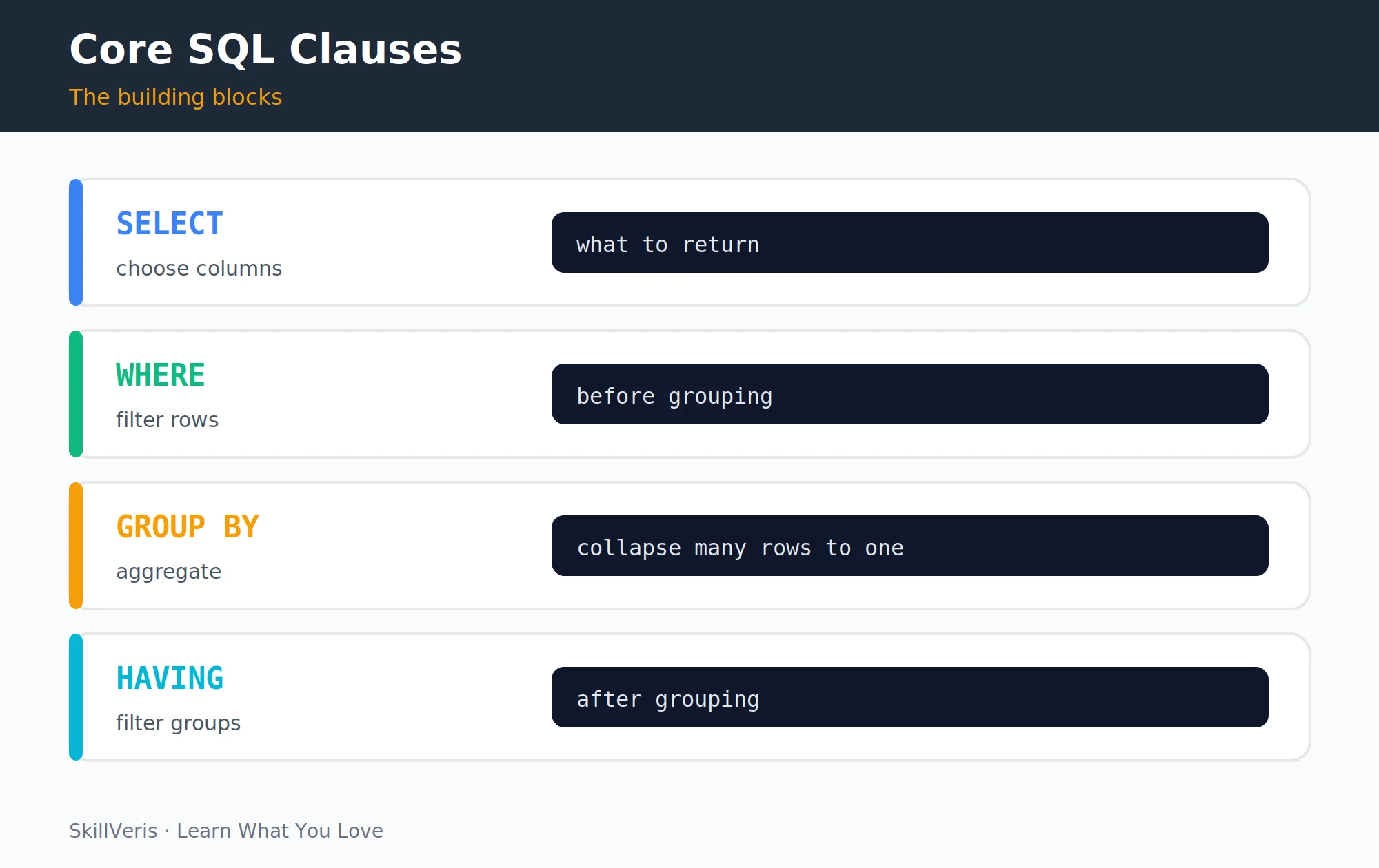
Grouping by team and player
Aggregate goals per home team and per goal scorer.
-- Goals scored by each team at home
SELECT home_team AS team,
  SUM(home_goals) AS goals_scored,
  COUNT(*) AS home_games
FROM matches
WHERE season = '2023/24'
GROUP BY home_team
ORDER BY goals_scored DESC;
-- Top goal scorers
SELECT player_id,
  COUNT(*) AS goals
FROM goals
WHERE goal_type != 'own goal'
GROUP BY player_id
ORDER BY goals DESC
LIMIT 10;7HAVING: Filter After Grouping
WHERE filters rows before grouping; HAVING filters groups after aggregation. This distinction trips up many beginners, because you cannot use an aggregate function such as COUNT or AVG inside WHERE.
HAVING lets you keep only the teams that averaged more than two goals per home game, or only the players with five or more goals.
Filtering groups
Use HAVING to filter on aggregated values.
-- Teams that averaged more than 2 goals per home game
SELECT home_team,
  AVG(home_goals) AS avg_home_goals
FROM matches
WHERE season = '2023/24'   -- filters rows BEFORE grouping
GROUP BY home_team
HAVING AVG(home_goals) > 2.0   -- filters groups AFTER aggregation
ORDER BY avg_home_goals DESC;
-- Players with 5+ goals (can't use WHERE here)
SELECT player_id, COUNT(*) AS goals
FROM goals
GROUP BY player_id
HAVING COUNT(*) >= 5
ORDER BY goals DESC;8JOIN: Combining Tables
The goals table stores player_id, not names, so a JOIN links goals to players to retrieve the name and team. JOIN is the most powerful SQL operation because it lets you answer questions that span multiple tables.
You can chain joins to combine matches, goals, and players into a single result, such as every Arsenal home match with its scorers and the minute each goal was scored.
Joining goals, players, and matches
Resolve player names and combine three tables in one query.
-- Top scorers with player names
SELECT p.name,
  p.team,
  COUNT(g.goal_id) AS goals
FROM goals g
JOIN players p ON g.player_id = p.player_id
WHERE g.goal_type != 'own goal'
GROUP BY p.player_id, p.name, p.team
ORDER BY goals DESC
LIMIT 10;
-- Match results with home and away goal scorers
SELECT m.date, m.home_team, m.away_team,
  m.home_goals, m.away_goals,
  p.name AS scorer, g.minute
FROM matches m
JOIN goals g ON m.match_id = g.match_id
JOIN players p ON g.player_id = p.player_id
WHERE m.home_team = 'Arsenal'
AND m.season = '2023/24'
ORDER BY m.date, g.minute;9Subqueries
A subquery is a SELECT nested inside another SELECT, useful for multi-step questions where one query depends on the result of another. A classic example finds players who scored more goals than the season average.
The inner query computes per-player goal counts, a wrapping query averages them, and the outer query keeps only players above that average.
Players above the average
Compare each player against a value computed by a subquery.
-- Players who scored more goals than the season average
SELECT p.name, COUNT(g.goal_id) AS goals
FROM goals g
JOIN players p ON g.player_id = p.player_id
GROUP BY p.player_id, p.name
HAVING COUNT(g.goal_id) > (
  SELECT AVG(goal_count)
  FROM (SELECT player_id, COUNT(*) AS goal_count
        FROM goals GROUP BY player_id) sub
)
ORDER BY goals DESC;10Window Functions (Intermediate)
Window functions perform calculations across a set of rows without collapsing them into groups, which makes them perfect for rankings and running totals. A RANK() with PARTITION BY ranks each player within their own team.
Because the rows are not collapsed, you keep every player's name alongside their rank.
Ranking within teams
Use RANK() OVER (PARTITION BY ...) to rank players per team.
-- Rank players by goals within each team
SELECT p.name, p.team,
  COUNT(g.goal_id) AS goals,
  RANK() OVER (
    PARTITION BY p.team
    ORDER BY COUNT(g.goal_id) DESC
  ) AS team_rank
FROM goals g
JOIN players p ON g.player_id = p.player_id
GROUP BY p.player_id, p.name, p.team
ORDER BY p.team, team_rank;11Putting It All Together: The League Table
The final challenge reconstructs the official league table entirely from raw match data. CASE WHEN expressions handle conditional logic inside aggregations, counting wins, draws, and losses and awarding points accordingly.
Conditional counting and summing inside aggregates is one of the most useful SQL patterns in business reporting, not just football analytics.
Building the table
CASE WHEN inside SUM rebuilds the standings from scratch.
-- Build the league table from raw match data
SELECT team,
  COUNT(*) AS played,
  SUM(CASE WHEN result = 'win' THEN 1 ELSE 0 END) AS wins,
  SUM(CASE WHEN result = 'draw' THEN 1 ELSE 0 END) AS draws,
  SUM(CASE WHEN result = 'loss' THEN 1 ELSE 0 END) AS losses,
  SUM(goals_for) AS gf,
  SUM(goals_against) AS ga,
  SUM(goals_for) - SUM(goals_against) AS gd,
  SUM(CASE WHEN result = 'win' THEN 3
           WHEN result = 'draw' THEN 1
           ELSE 0 END) AS points
FROM team_results   -- a view combining home and away
WHERE season = '2023/24'
GROUP BY team
ORDER BY points DESC, gd DESC, gf DESC;12Key Takeaways
These five clauses, joined together, answer almost any question you can ask of a football dataset, and the same patterns transfer directly to business reporting.
- SQL query order: SELECT to FROM to JOIN to WHERE to GROUP BY to HAVING to ORDER BY to LIMIT.
- WHERE filters rows; HAVING filters groups. You can't use aggregate functions in WHERE.
- JOIN links tables by a shared key and is the most powerful SQL operation.
- CASE WHEN inside an aggregate function enables conditional counting and summing.
- Football data is a perfect learning context because every query answers a question you actually want answered.
13What to Learn Next
Apply your new SQL skills in a broader analytics context and connect them to Python and APIs.
- Data Analytics Roadmap: see where SQL fits in the full analyst stack.
- Pandas for Beginners: the Python alternative for the same operations.
- Build a REST API: use SQL to back a FastAPI endpoint.
14Frequently Asked Questions
Which SQL database should I use to practise? Use SQLite for local practice since it needs no server, is free, and ships with Python. PostgreSQL is best for production-realistic practice, and MySQL is also common. The SQL syntax in this guide works in all three with minimal changes.
Where can I find free football SQL datasets? Kaggle has several Premier League and European league datasets. StatsBomb provides free open data including detailed event data from selected competitions, and Football-data.co.uk offers match results going back decades as free CSVs.
What is the difference between INNER JOIN, LEFT JOIN, and RIGHT JOIN? INNER JOIN returns only rows that match in both tables. LEFT JOIN returns all rows from the left table plus matched rows from the right, with nulls where there is no match, and RIGHT JOIN is the mirror. Start with INNER JOIN, and use LEFT JOIN when you want to keep all rows from one table even without a match in the other.
Is SQL case-sensitive? SQL keywords such as SELECT, FROM, and WHERE are case-insensitive by convention, with uppercase being standard for readability. String comparisons depend on the database and collation setting; in SQLite they are case-sensitive by default, so use LOWER(team) = 'arsenal' to make them case-insensitive.
Related Reading
Get The Print Version
Download a PDF of this article for offline reading.
About the Publisher
SkillVeris Team
Content Team
We believe the best way to learn tech is through what you already love — sports, music, photography, and more.
View all postsRelated Posts
Never miss an update
Get the latest tutorials and guides delivered to your inbox.
No spam. Unsubscribe anytime.